How to Analyze a Graph: Step by Step Guide, 4 Examples

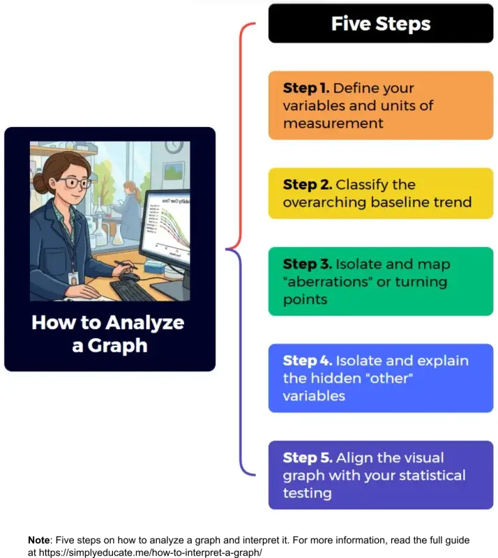
How do you analyze a graph? This article provides a step-by-step procedure on how to analyze a graph.

To illustrate the key principles applied, four illustrative examples are given.

Introduction

My undergraduate students would occasionally approach me and consult on some of the difficulties they encountered while preparing their thesis.

One of those things that they usually ask me is how they should go about the graphs in the results and discussion section of their paper.

Are you struggling to understand how to interpret a graph effectively just like them?

Graph interpretation is easy if you have a basic foundation.

This guide breaks down essential techniques that will transform you from confused to a confident interpreter of research data analyzed using the graph function of the ubiquitous MS Excel or other spreadsheet applications. You can then choose which trendline most fits your data.

This article will help you extract meaningful insights and communicate data findings with clarity and impact.

How should the graphs and the table be interpreted by the thesis writer?

Here are the steps on how to analyze graphs—in very simple terms—using only two variables to show relationships.

5 Step-by-Step Procedure on How to Analyze Graphs and Interpret Them

Step 1: Define your variables and units of measurement

Before interpreting what the data means, clearly define what the graph is measuring.

• What to do: Identify your horizontal axis (x-axis) or abscissa and vertical axis (y)-axis) or ordinate. State their operational names and units of measurement.
• What to write in your draft: “Figure [X] shows the relationship between [Variable A, x-axis] measured in [e.g., hours/km/psi] and [Variable B, y-axis] measured in [e.g., scores/liters/currency].”

Step 2: Classify the overarching baseline trend

Look at the general trajectory of the data from left to right to determine the underlying relationship.

• Direct / Positive Correlation: If one variable increases and the other increases alongside it, they are directly related.
• Inverse / Negative Correlation: If one variable increases while the other decreases in proportionate amounts, they share an indirect relationship.
• Unrelated Data: If the scatter points or lines show no cohesive pattern, shape, or trajectory, use your training to accept that the variables are likely unrelated. Do not force a correlation where none exists.

Step 3: Isolate and map “aberrations” or turning points

Real-life research data rarely forms a perfectly straight line. Look for deviations from the general trend.

• What to do: Identify unexpected peaks, sharp drops, plateaus (saturation points), or sudden shifts in the direction of the curve.
• What to write in your draft: “While the overall trend shows a progressive increase, a noticeable aberration occurs between [Point A] and [Point B], where the values temporarily decline/plateau.”

Step 4: Identify and Explain the Hidden “Other” Variables

When a trend line shifts unexpectedly, it is usually influenced by outside factors not plotted on the axes. This is where your critical thinking, reading, and imagination come into play.

• What to do: Uncover the external catalyst causing the anomaly (e.g., an economic recession causing a dip in profits, environmental pollution causing a drop in tourism, or a change in testing conditions).
• What to write in your draft: “This specific aberration is likely influenced by [insert external variable or factor], which temporarily altered the expected interaction between [Variable A] and [Variable B].”

Step 5: Align the Visual Graph with Your Statistical Testing

Never rely on automated statistical printouts (like the Excel Analysis ToolPak) without looking at your plotted data first to avoid spurious generalizations.

A spurious generalization is a broad conclusion or rule that is fundamentally false, invalid, or incorrect because it is built on a “spurious correlation”—meaning, the relationship between the things being observed is purely coincidental, deceptive, or caused by an unseen third variable (see confounding variables in my post: Identifying Variables for Your Research Paradigm: A Guide for Graduate Researchers.

• What to do: Ensure that the peaks, valleys, or straight lines seen on your graph match the story told by your t-test, F-test, or p-values. The visual graph should serve as the clear, illustrative proof of your statistical data.

How to Analyze a Graph: 4 Illustrative Examples

Based on the key principles mentioned a while ago, I explain the procedure using concrete examples with illustrations in this section.

Graphs are powerful illustrations of relationships between the variables of your study. They can show whether the variables are directly related, inversely related, or show something else.

I illustrate the common situations encountered by a researcher namely direct or positive relationship, inverse or negative relationship, and neither direct nor inverse but some relationship is shown.

These interpretations provide foundational knowledge on interpreting a graph, the common xy situation where you see, in Math lingo, the abscissa (horizontal or x-axis) and the ordinate (vertical or y-axis).

1. Direct, Positive Relationship

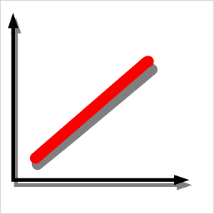
This relationship between variables is visually represented in Figure 1. If one variable increases in value, the other variable increases as well, indicating a direct relationship.

This relationship between variables is also called positive correlation, direct correlation, positive association, direct proportionality, linear relationship, or direct variation.

For example, if you pump air into a tire, the tire expands, and so does the air pressure inside it to hold the rubber up. This is the pressure-volume relationship, a classic example from physics and chemistry.

The variables in this relationship are pressure and volume. Pressure may be measured in pounds per square inch (psi), and volume in liters (L) or cubic centimeters (cm³).

If pressure is increased, there is a corresponding increase in volume. The two variables are directly related.

Here are a few more examples:

1. Temperature and volume of a gas (Charles’s Law): As temperature increases, the volume of a gas expands, assuming pressure remains constant.
2. Speed and distance traveled (assuming constant time): The faster you move, the greater the distance you cover in a given time.
3. Study time and exam score: Generally, the more time you spend studying, the higher your exam score (assuming effective study methods).

These examples highlight how graphs can visually represent and clarify the relationships between variables in various scientific, mathematical, and real-world contexts.

2. Inverse Relationship

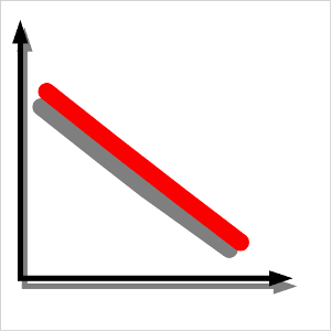
How about if you have another graph like the one at right (Figure 2)?

Well, it’s just as simple as the first one. If one variable increases in value, the other variable decreases in proportionate amounts. This graph shows an inverse relationship between the two variables. This relationship between variables is also described as negative correlation or indirect relationship.

For example, as a driver increases the speed of the vehicle he or she is driving, the time it takes to reach the destination decreases. Of course, this assumes that there are no obstacles along the way. The variables involved in this relationship are speed and time. Speed may be measured in kilometers per hour (km/hr), and time in hours.

Here are a few more examples of inverse relationships:

1. Price and demand: As the price of a product increases, the demand for it often decreases, assuming all other factors remain constant.
2. Battery charge and usage time: The more you use a device, the faster the battery drains. So, battery life decreases as usage increases.
3. Distance from a light source and brightness: The farther you are from a light source, the dimmer it appears. This is an inverse relationship between distance and brightness.

These examples illustrate how inverse relationships can be observed in economics, everyday life, and science.

The two examples of graphs given are very simplified representations of the relationship between two variables. In many studies, these relationships seldom occur. Graphs show something else. Not really straight lines but curves.

Let’s proceed to the next section to discuss this situation.

3. Neither Strictly Direct Nor Inverse Relationship

In real life, the relationship between variables shows neither a direct relationship nor an inverse relationship. If you use a scatter graph, for example, you might encounter something different. These situations often occur when dealing with many samples, where a trend over time could be discerned.

And note this: using scatter graph is a powerful tool to understand your data before making interpretations or conclusions about it. Sometimes, students just interpret the output in their statistical software applications like the easily accessible Excel Analysis ToolPak without plotting the data first. They are then prone to committing spurious generalizations.

Excel Analysis ToolPak: Example Data Analysis of 18 Samples Using t-test

For example, how will you interpret the two graphs below (Figure 3, Graphs a and b)? Some students have trouble interpreting these.

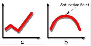
Graph a actually shows that the relationship between the two variables goes up and down before progressively increasing. In general, the relationship is directly proportional over time.

Graph a may show the relationship between a company’s profit over time. The vertical axis represents profit, while the horizontal axis represents time. The graph portrays that initially, the profit increased, but at a certain point in time, it decreased. After that, the profit recovered and continued to increase throughout the period.

Such fluctuations may be caused by various factors. For example, the profit of the company may have declined due to a recession. However, once the recession ended, profits continued to increase, and things gradually improved over time.

Here are a few more examples of similar situations:

• Stock market performance: A stock’s value may rise and fall over time due to market fluctuations, but eventually trend upward as the company becomes more stable or profitable.
• Population growth in a city: A city’s population may initially grow rapidly, then decline due to economic downturns or migration, before increasing again as the economy improves.
• Sales of a new product: Sales may start high due to initial interest, then drop as the novelty wears off, but eventually rise again as the product becomes more established or receives positive reviews.

These examples illustrate how real-world data can show complex patterns that are not strictly direct or inverse, but still follow a general trend over time.

How about Graph b?

Graph b simply means that a variable in question reaches a saturation point. This graph may represent the number of tourists visiting a popular island resort over time. Within the span of the study—say, 10 years—at about five years since the beach resort started operating, the number of tourists reached a peak and then began to decline. The reason may be a polluted coastal environment that caused tourists to shy away from the place.

Here are a few more examples of similar situations:

1. Adoption of a new technology: Initially, the number of users increases rapidly as the technology gains popularity. However, after a certain point, the growth slows and eventually plateaus as the market becomes saturated.
2. Sales of a new product: A product may see a surge in sales at first, but as the market becomes saturated, demand decreases, and sales begin to decline.
3. Population growth in a region: A region may experience rapid population growth due to economic opportunities, but as resources become limited or the environment degrades, the population growth may slow or even decline.

These examples show how variables can reach a peak and then decline due to external or internal factors, such as environmental issues, market saturation, or resource limitations.

These situations lead to other trendline variations shown in the next section. Basically, these variations are combinations of the first two examples.

4. Other Trendline Variations

There are many  variations in the relationship between two variables. It may look like an S curve going up or down, plain horizontal line, or U-shaped, among others.

Those are actually just variations of direct and inverse relationship between the two variables. They require curve fitting, to approximate the general direction of the trend.

For this reason, the final interpretation requires the researcher’s incisive look into the scatter plot to make sense of relationships. This capability depends on the the researcher’s experience and insightful thinking.

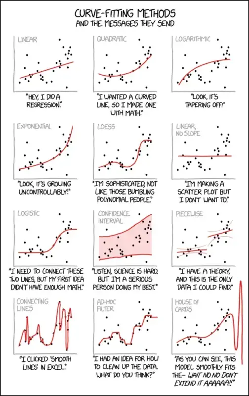
Just note that aberrations along the way are caused by something else — another variable or set of variables or factors that affect one or both variables, which you need to identify and explain.

Or, if you cannot interpret the graph in any other way and you believe the variables are related, then you have to accept the fact that they are, in fact, unrelated.

That’s where your training, imagination, experience, and critical thinking come in. Interpreting graphs need not be difficult if you know the basics.

---

Frequently Asked Questions (FAQs)

Interpreting a graph is not difficult as long as you are equipped with this knowledge. Keep practicing!

©SimplyEducate.me | Patrick Regoniel